Introduction
Before a machine can understand the content of an image or detect its liveness, it must first learn to see its structure. That’s why in the vast field of computer vision, edge detection in image processing is considered one of the most fundamental and powerful operations today. With edge detection, a machine can identify sharp changes in pixel intensity – "edges" – that often correspond to object boundaries. This guide breaks down the essential theory, compares the most influential algorithms, and offers expert answers to common questions. Let’s start with the basic definition.
What is Edge Detection in Image Processing?
Definition : Edge detection is a process used to find significant transitions in brightness within an image. These transitions represent the contours or outline of objects. According to Gonzalez & Woods (Digital Image Processing, 4th Edition), edge detection simplifies visual data by reducing dimensionality and revealing geometric structures critical for interpretation.
In simple terms, Edge detection helps a computer "see" the structure of a scene by finding where one object ends and another begins. When an image is being processed, edge detection converts a complex, pixel-rich image into a cleaner set of edge contours, and reduces the computational overhead required for more advanced tasks, such as object recognition, image segmentation, and 3D reconstruction.
The goal of edge detection in image processing is to produce a simplified edge map that preserves the structural properties of a scene while dumping irrelevant information. These edges occur at the outline that separates a person from their background, the transition from a smooth wall to a textured carpet or the distinct line cast by a shadow.

Native approach to detecting edges starts with simply running through all the pixels – determining whether we see a large jump in intensity compared to its neighbours.
A study published in Nature Biomedical Engineering (2019) found that incorporating edge-enhanced pre-processing improved tumour segmentation accuracy by 5.8% in deep learning models.
How Edge Detection Improves Facial Recognition?
Edges are where information density is highest. They define object shape, orientation, and spatial relationship. In many vision pipelines, edge detection is the first stage before segmentation, classification, or 3D reconstruction.
For example:
In medical imaging, edges help detect the outline of a tumour.
In self-driving cars, they reveal lane markings or road boundaries.
In biometric systems, they define key facial landmarks.
Without accurate edge detection, most vision-based AI systems would struggle to understand what they're seeing.
With the help of coherent gating liveness detection, Mantra integrates classical edge detection into its facial recognition pipeline. Sobel and Canny filters are applied during preprocessing to enhance the structural clarity of facial features.
Here’s how it works:
-
Preprocessing
An incoming video frame is first passed through a Canny edge detector. This creates a clean structural map of the face, highlighting the jawline, eye sockets, and nose bridge.
-
Feature Fusion
This edge map is fed into the Mantra deep learning model as an additional input channel, alongside the standard RGB image.
-
Robust Inference
The model now uses both the visual texture (from RGB) and the explicit structure (from the edge map) to locate facial landmarks. This hybrid approach makes the system far more resilient to challenges like poor lighting or face masks, where RGB data alone might fail.
What are the Main Edge Detection Algorithms?
The most widely used edge detection algorithm is the Canny edge detector, developed by John Canny in 1986. Despite decades of newer methods, his algorithm remains the gold standard due to its precision and noise resilience.
Before diving into edge detection algorithms, it's essential to understand convolution - the core mathematical process behind most edge detection algorithms.
Convolution involves sliding a small matrix – called a kernel – across an image and computing a weighted sum of the overlapping pixels. To perform this operation correctly, the kernel is typically flipped both horizontally and vertically, then multiplied element-wise with the corresponding region of the image matrix. The resulting products are summed to yield a single value, which becomes the output for that pixel location.
Furthermore, some of the most advanced edge detection algorithms look for steep changes through changes in convolution. As mentioned earlier, each of the following offers a different balance of performance and computational cost.
Let’s break down each edge detection algorithm one by one:
-
The Prewitt Operator
The Prewitt operator is a straightforward, gradient-based method. Gradient is a measure of how quickly the pixel values are changing. Think of it as the filter pointing out where the image shifts from light to dark or vice versa.
Prewitt uses two small 3x3 kernels (small grids of numbers) to scan the image, one for horizontal edges and one for vertical. It’s computationally inexpensive but susceptible to noise, making it suitable for clean images in controlled environments. So “gradient-based” methods like Prewitt are all about finding spots where the brightness jumps – this usually means there’s an edge.
Prewitt Kernels:
Gx = [[-1, 0, 1], [-1, 0, 1], [-1, 0, 1]]
Gy = [[1, 1, 1], [0, 0, 0], [-1, -1, -1]]
Here, Gx represents horizontal changes (changes going left to right), whereas Gy represents vertical changes (changes going up and down).
-
The Sobel Operator
Developed by Irwin Sobel and Gary Feldman at the Stanford Artificial Intelligence Laboratory (SAIL) in 1968, the Sobel operator is a cornerstone of edge detection in image processing since it calculates the approximate gradient of the image intensity at each point by convolving the image with two 3x3 kernels. Thus, the Sobel operator improves on Prewitt by giving more weight to the central pixels in its kernel. This makes it more robust to noise while still computationally efficient.
Sobel Kernels:
Gx = [[-1, 0, 1], [-2, 0, 2], [-1, 0, 1]]
Gy = [[-1, -2, -1], [0, 0, 0], [1, 2, 1]]
-
The Laplacian of Gaussian (LoG)
Instead of finding the peak gradient, the LoG operator (also known as the Marr-Hildreth algorithm) finds edges by looking for zero-crossings in the second derivative of the image. It first smooths the image with a Gaussian filter and then applies the Laplacian operator. This method is excellent at detecting fine, well-localised edges but can be sensitive to noise.
Note: To enhance contrast and suppress noise, a normalisation step is typically applied. This involves dividing all gradient values by the maximum gradient magnitude observed across the image. The result is a visually interpretable map that highlights object boundaries with greater clarity.
| Algorithm | Speed | Noise Robustness | Edge Localization | Best Use Cases |
|---|---|---|---|---|
| Prewitt | 5 out of 5 stars | 2 out of 5 stars | 2 out of 5 stars | Educational purposes |
| Sobel | 4 out of 5 stars | 3 out of 5 stars | 3 out of 5 stars | Real-time image processing |
| LoG | 3 out of 5 stars | 2 out of 5 stars | 4 out of 5 stars | Medical & scientific imaging |
| Canny | 2 out of 5 stars | 5 out of 5 stars | 5 out of 5 stars | Production systems, automation |
Data based on benchmarking results from OpenCV and MathWorks MATLAB labs
How does the Canny Algorithm work?
The Canny edge detector is not a single step but a multi-stage algorithm designed to maximise edge quality. Let’s break down its four critical stages:
-
Blurring Noise Reduction
All real-world images contain some noise. Since edge detection is based on derivatives, it is highly susceptible to noise. The Canny algorithm begins by applying a Gaussian filter to smooth the image and suppress these random fluctuations without overly damaging the structural edges.
-
Finding Intensity Gradients
Once the image is smoothed, the algorithm calculates the gradient magnitude and direction for every pixel using Sobel filters, just like the Sobel operator. This step produces a map of potential edges, but they are thick and noisy.
-
Non-Maximum Suppression
This is the clever step that thins the thick edges into sharp, single-pixel lines. For each pixel, the algorithm looks at its neighbours in the positive and negative gradient direction. If the pixel’s gradient magnitude is not the absolute maximum compared to its neighbours along that line, it is suppressed (set to zero). The result is a map of sharp, “candidate” edges.
-
Hysteresis Thresholding
This final stage is what truly sets Canny apart. It uses two thresholds - a high and a low - to differentiate real edges from noise.
Any pixel with a gradient magnitude above the high threshold is immediately confirmed as a “strong” edge.
Any pixel below the low threshold is immediately discarded.
Any pixel between the two thresholds is marked as a “weak” edge. It is only confirmed as a real edge if it is connected to a “strong” edge.
This hysteresis process allows the canny edge algorithm to trace along faint but real edges, creating continuous contours while ignoring isolated noise pixels.
First and Second Derivatives in Edge Detection Explained
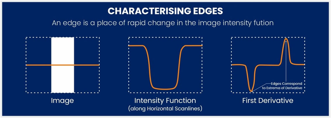
Edge detection relies on the mathematical concept of derivatives to quantify how image intensity changes over space and therefore, falls into two major categories: first-order derivative methods (detecting sharp intensity changes) and second-order derivative methods (detecting zero-crossings). Each method varies in complexity, noise sensitivity, and quality of results and is based on a simple mathematical concept: finding where the image’s intensity function has a high first derivative.
The first derivative captures how rapidly pixel values change, which is essential for identifying boundaries where objects in an image differ in brightness. High values in the first derivative signal strong intensity gradients - an indicator of an edge. Common gradient-based operators such as Sobel, Prewitt, and Scharr are practical implementations that approximate this first derivative in both horizontal and vertical directions.

The yellow line shows the edges of an outline working at three different scenarios.
In contrast, the second derivative looks at how the rate of change itself varies. It doesn't just detect where intensity shifts, but where those shifts accelerate or decelerate. This makes it valuable for identifying zero-crossings - points where the second derivative transitions from positive to negative or vice versa, often aligning closely with true edge locations. The Laplacian operator is a standard method for approximating the second derivative in image processing.
Together, these derivative-based approaches form the foundation of most edge detection techniques used in medical imaging, satellite vision, and AI-powered object recognition systems.
Conclusion
While deep learning models like CNNs automatically learn feature hierarchies, classical edge detection in image processing has found a new role as a critical complementary technique. From the simple Prewitt operator to the sophisticated Canny algorithm, edge detection in image processing remains a cornerstone in face detection APIs. The most advanced AI solutions today do not replace these fundamentals - they build upon them, proving that a solid foundation is the key to innovation.
FAQs
An edge is a local intensity change; a boundary represents a separation between distinct regions or objects. Edge detection helps identify boundaries.
It uses two thresholds. Strong edges (above high) are kept, weak edges (between thresholds) are only kept if connected to strong ones. This reduces noise while preserving real edges.
Yes. Edge detection principles apply to 3D point clouds by analysing changes in depth, surface normals, or density.
Noise, lighting variations, or compression artefacts can create false intensity changes mistaken for edges. Noise filtering is essential.
Usually, images are converted to grayscale first. Alternatively, edges can be detected in each RGB channel separately and combined.
Thresholds depend on the image. Low thresholds detect more but may include noise. High thresholds detect fewer, stronger edges. Canny’s dual-threshold approach handles this more effectively.
Comments